
Charts, Graphs & Healthcare Data Visualization
Week 5 — Lesson 1 | CI2000: Computer Fundamentals
Learning Objectives
- Given a healthcare dataset, create column, bar, line, and pie charts that accurately represent the data relationships and include professional titles, labels, and legends (CO-6)
- Select the most appropriate chart type for a given data relationship (comparison, trend, composition, or distribution), justifying the choice based on the story the data needs to tell (CO-7)
- Customize chart elements — titles, legends, data labels, axes, and colors — to produce publication-ready visualizations suitable for a healthcare board report (CO-6)
- Interpret a healthcare data visualization to identify key findings, trends, or anomalies that inform clinical or administrative decision-making (CO-7)
Part 1: Why Data Visualization Matters in Healthcare
Healthcare organizations generate massive volumes of data every day — patient visits, lab results, billing transactions, staffing hours, supply orders, and outcomes measurements. Raw numbers in a spreadsheet can be overwhelming and difficult to interpret, especially when a clinic manager or administrator needs to make a decision quickly. This is where data visualization becomes essential.
A chart or graph transforms rows and columns of numbers into a visual picture that reveals patterns, trends, and outliers at a glance. Consider the difference between scanning 500 rows of monthly patient-visit data versus glancing at a line chart that clearly shows a seasonal spike in visits every January. The chart communicates the same information in seconds rather than minutes.
The Role of Charts in Healthcare Decision-Making
In healthcare settings, data visualizations support critical functions across five key areas. Explore each one:
Clinical quality improvement — Tracking patient outcomes, readmission rates, and infection rates over time to identify areas for improvement.
Example: A line chart showing monthly surgical site infection rates over 18 months reveals whether a new sterilization protocol is reducing infections.
Financial management — Comparing revenue to expenses across departments, monitoring insurance claim denial rates, and forecasting budget needs.
Example: A column chart comparing quarterly revenue vs. expenses across Cardiology, Orthopedics, and Primary Care highlights which departments are most profitable.
Operational efficiency — Visualizing patient wait times, appointment no-show rates, and room utilization to optimize scheduling.
Example: A bar chart of average wait times by day of week reveals that Mondays have 40% longer waits, prompting staffing adjustments.
Regulatory compliance — Generating charts for accreditation audits, quality reporting programs like HEDIS and MIPS, and public health reporting.
Example: A dashboard with pie charts showing immunization rates by age group provides instant proof of compliance for a state health department audit.
Population health — Identifying disease trends in patient populations, tracking vaccination rates, and monitoring chronic disease management outcomes.
Example: A scatter chart plotting A1C levels against BMI for a diabetes population reveals the correlation between weight management and glucose control.
Healthcare Connection: A clinic quality coordinator uses a line chart to track monthly patient satisfaction scores over the past two years. The chart immediately reveals a downward trend that started six months ago, prompting an investigation into staffing changes that coincided with the decline. Without the chart, this pattern might have gone unnoticed in the raw survey data.
Part 2: Chart Types and When to Use Each
Excel offers a wide variety of chart types, but choosing the right one is critical. An inappropriate chart type can distort the data or make it harder to understand. The key is to match the chart type to the relationship you want to show in your data. There are four fundamental data relationships, and each one maps to specific chart types.
Click each chart type below to learn when to use it and see a healthcare example:
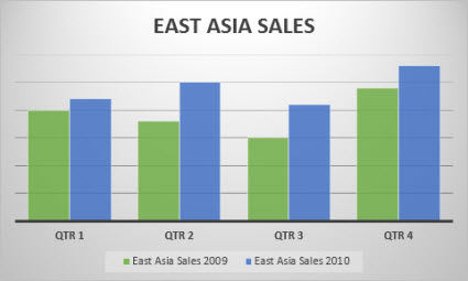
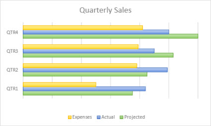
Comparison: Column & Bar Charts
Use column charts and bar charts when you want to compare values across categories. A column chart uses vertical bars, while a bar chart uses horizontal bars. Column charts work well when you have a small number of categories and short labels. Bar charts are better when you have many categories or long category names that would overlap on a horizontal axis.
Healthcare example: A column chart comparing the number of patient visits by department (Cardiology, Orthopedics, Primary Care, Pediatrics, OB/GYN) during a single quarter makes it easy to see which departments are busiest.
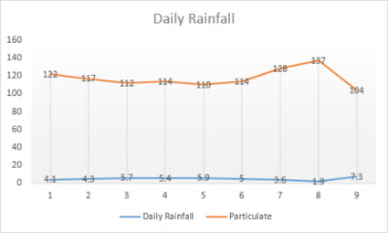
Trend Over Time: Line & Area Charts
Line charts connect data points with a continuous line, making them ideal for showing how a value changes over time. Each point represents a measurement at a specific time interval. Area charts are similar but fill the area below the line with color, useful for showing the magnitude of change or comparing cumulative totals.
Healthcare example: A line chart tracking monthly emergency department visits over 24 months reveals seasonal patterns — spikes during flu season in winter and a dip during summer months.
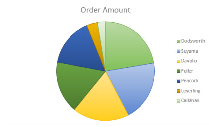
Composition: Pie & Doughnut Charts
Pie charts show how parts make up a whole. Each slice represents a category's percentage of the total. Pie charts work best with a small number of categories (ideally 5 or fewer) and when one or two categories clearly dominate. Doughnut charts are similar but include a hollow center.
Healthcare example: A pie chart showing the percentage breakdown of insurance types (Medicare 35%, Commercial 30%, Medicaid 20%, Self-Pay 10%, Other 5%) gives a quick view of the payer mix.
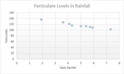
Distribution & Relationship: Scatter Charts
Scatter charts (also called XY charts) plot individual data points using two numeric axes to show the relationship or correlation between two variables. They are particularly valuable in research and clinical quality analysis.
Healthcare example: A scatter chart plotting patient wait time on the X-axis against patient satisfaction score on the Y-axis can reveal whether longer wait times correlate with lower satisfaction ratings.
Multiple Relationships: Combination Charts
Combination (combo) charts merge two chart types — typically a column chart and a line chart — on the same axes. This is useful when you have two data series measured on different scales.
Healthcare example: A combo chart showing monthly patient volume as columns (left axis) and average wait time as a line (right axis) allows administrators to see whether increased volume drives longer wait times.
Pro Tip: When in doubt, ask yourself: "What relationship am I trying to show?" Comparison = column/bar. Trend = line. Composition = pie. Correlation = scatter. Two scales = combo. This simple decision tree will guide you to the right chart type every time.
Chart Selection Quick-Reference Guide
| Chart Type | Data Relationship | Best For | Healthcare Example |
|---|---|---|---|
| Column Chart | Comparison | Comparing values across a small number of categories | Patient visits by department in Q1 |
| Bar Chart | Comparison | Comparing values when category labels are long or numerous | Top 15 diagnosis codes by frequency |
| Line Chart | Trend over time | Showing change across continuous time intervals | Monthly ER visits over 24 months |
| Area Chart | Trend / cumulative | Showing magnitude of change or stacked totals over time | Cumulative vaccine doses administered by week |
| Pie Chart | Composition | Showing parts of a whole (5 or fewer categories) | Insurance payer mix: Medicare, Medicaid, Commercial, Self-Pay |
| Scatter Chart | Correlation / distribution | Revealing relationships between two numeric variables | Wait time vs. patient satisfaction scores |
| Combination Chart | Multiple relationships | Displaying two data series on different scales together | Monthly patient volume (columns) + average wait time (line) |
| Sparkline | Trend (compact) | Showing a mini trend within a single cell | Inline trend of daily appointments per provider row |
▶ Pivot Table Excel Tutorial • Kevin Stratvert
Part 3: Creating Charts from Healthcare Data in Excel
Creating a chart in Excel follows a consistent workflow regardless of the chart type. According to Microsoft's official documentation, the process involves selecting your data, inserting a chart, and then customizing its appearance. Let's walk through this process using a realistic healthcare scenario.
Expand each step below to learn the complete chart creation workflow:
Step 1: Prepare Your Data
Good charts start with well-organized data. Your data should be arranged in rows and columns with clear headers. For most charts, each column represents a data series and each row represents a category or time period. Avoid blank rows or columns within your data range.
Scenario: You manage the front office for a multi-specialty clinic. Your spreadsheet tracks monthly patient visits by department for the past six months:
- Column A: Month (January through June)
- Column B: Primary Care visits
- Column C: Cardiology visits
- Column D: Orthopedics visits
- Column E: Pediatrics visits
Step 2: Select the Data Range
Click and drag to select the entire data range including headers. In our example, you would select the range A1:E7 (headers plus six months of data across four departments). Excel uses the headers to automatically label your chart series and categories.
Step 3: Insert the Chart
Navigate to the Insert tab on the Ribbon. In the Charts group, select Column Chart and choose Clustered Column. Excel instantly generates a chart with each department as a different colored bar and each month on the horizontal axis.
Alternatively, select Recommended Charts to let Excel analyze your data and suggest the most appropriate chart types.
Step 4: Position and Resize
The new chart appears as a floating object on your worksheet. Click and drag it to position it below or beside your data. Use the corner handles to resize. For a polished look, align the chart edges with your data columns.
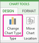
Chart Sheets vs. Embedded Charts
By default, Excel creates an embedded chart on the same worksheet as your data. For a full-page chart for printing, right-click the chart and select Move Chart → New Sheet. Chart sheets are ideal for meeting handouts and printed reports.
Healthcare Connection: A practice administrator creates a clustered column chart showing patient visits by department for six months. At the monthly management meeting, the chart immediately reveals that Primary Care visits spiked in March during flu season while Orthopedics remained flat. This insight drives a discussion about seasonal staffing adjustments.
Try It Yourself: Open a blank Excel workbook and enter monthly patient visit data for three departments across six months. Select the data range, click Insert → Column Chart → Clustered Column, and watch Excel create the chart instantly. Then try Recommended Charts to see what Excel suggests.
Part 4: Customizing Chart Elements for Professional Presentations
A default chart generated by Excel is functional but rarely presentation-ready. Customizing chart elements transforms a basic chart into a clear, professional visualization. Select each element below to learn how to customize it:
Chart Title: Every chart should have a descriptive title that tells the viewer exactly what data is being displayed. Select the default "Chart Title" text and type a specific, informative title.
Best practice: Use "Monthly Patient Visits by Department: January–June 2026" rather than a vague label like "Patient Data." Include the time period and what is being measured.
Axis Titles: Label the horizontal (category) and vertical (value) axes so the viewer understands the units. Click the + (Chart Elements) button and check Axis Titles.
Example: Horizontal axis = "Month" and vertical axis = "Number of Patient Visits." Without axis titles, viewers must guess what the numbers represent.
Legend: Identifies which color corresponds to each data series. By default, Excel places the legend at the bottom. You can reposition it to the right, top, or left.
Best practice: When a chart has many series, placing the legend on the right side provides the best readability. For single-series charts, consider removing the legend entirely to reduce clutter.
Data Labels: Display the exact numeric value on or near each data point. Useful when precision matters — for example, when presenting patient counts to administrators who need exact numbers.
Best practice: Data labels can clutter a chart with many data points. Use them selectively — perhaps only on the highest and lowest values, or only on the final data point in a trend line.
Gridlines: Horizontal or vertical lines extending from the axis, helping the viewer estimate values. Excel includes major horizontal gridlines by default.
Best practice: In healthcare presentations, keep major gridlines so stakeholders can read approximate values. Remove gridlines entirely for a cleaner look in executive presentations.
Formatting Colors & Styles: Excel's Chart Styles gallery on the Design tab offers pre-built color schemes. You can also right-click individual elements and select Format.
Best practice: Use your organization's brand colors for consistency. For UMA-branded materials, use navy (#1d6ba6) as primary and teal (#00b4d8) as secondary. A clean white background with readable fonts works best.
- Chart title — describes what the chart shows
- Plot area — the region where data is displayed
- Legend — identifies what each color or series represents
- Axis titles — labels describing what each axis measures
- Axis labels — the category names or values along each axis
- Tick marks — small marks along the axes indicating scale intervals
- Gridlines — horizontal or vertical lines that help read values accurately
Healthcare Connection: When preparing a chart for a regulatory audit or accreditation review, attention to detail matters. A clearly titled chart with proper axis labels, a legend, and consistent formatting demonstrates professionalism and makes the data easier for reviewers to evaluate. Poorly formatted charts can raise questions about data accuracy, even if the underlying numbers are correct.
Part 5: Conditional Summarization: SUMIF, COUNTIF, and AVERAGEIF
Before you create a chart, you often need to summarize raw data into meaningful categories. Healthcare spreadsheets frequently contain hundreds or thousands of rows. Excel's conditional summarization functions let you total, count, or average values based on specific criteria, creating the summary data that feeds your charts.
Explore each function to learn its syntax, purpose, and a healthcare application:
SUMIF — Sum Values That Meet a Condition
The SUMIF function adds up values in a range where a corresponding range meets a criterion.
Syntax: =SUMIF(range, criteria, [sum_range])
- range – The range evaluated against the criteria (e.g., department names).
- criteria – The condition that determines which cells to sum (e.g., "Cardiology").
- sum_range – The range of cells to add up when the criteria is met.
Healthcare example: To find the total charges for Cardiology:
=SUMIF(B:B, "Cardiology", D:D)
This scans column B and adds the corresponding value from column D whenever it finds "Cardiology."
COUNTIF — Count Entries That Meet a Condition
The COUNTIF function counts the number of cells in a range that meet a criterion.
Syntax: =COUNTIF(range, criteria)
- range – The range of cells to count.
- criteria – The condition that determines which cells are counted.
Healthcare example: To count patient visits to Pediatrics:
=COUNTIF(B:B, "Pediatrics")
Use this for each department to create a summary table that feeds a column chart comparing visit volumes.
AVERAGEIF — Average Values That Meet a Condition
The AVERAGEIF function calculates the average of values where a corresponding range meets a criterion.
Syntax: =AVERAGEIF(range, criteria, [average_range])
Healthcare example: To find the average ER wait time:
=AVERAGEIF(B:B, "Emergency", E:E)
Where column B contains department names and column E contains wait times in minutes.
Pro Tip — Building chart-ready summaries: Create a small summary table using COUNTIF for visit counts, SUMIF for total charges, and AVERAGEIF for average wait times by department. This summary table becomes the data source for multiple charts on a performance dashboard.
Conditional Summarization Quick Reference
| Function | Syntax | Purpose | Healthcare Example |
|---|---|---|---|
| SUMIF | =SUMIF(range, criteria, sum_range) | Adds values where a condition is met | =SUMIF(B:B, "Cardiology", D:D) totals Cardiology charges |
| COUNTIF | =COUNTIF(range, criteria) | Counts cells where a condition is met | =COUNTIF(B:B, "Pediatrics") counts Pediatrics visits |
| AVERAGEIF | =AVERAGEIF(range, criteria, avg_range) | Averages values where a condition is met | =AVERAGEIF(B:B, "Emergency", E:E) averages ER wait times |
| SUMIFS | =SUMIFS(sum_range, r1, c1, r2, c2) | Adds values where multiple conditions are met | =SUMIFS(D:D, B:B, "Cardiology", C:C, "Medicare") |
| COUNTIFS | =COUNTIFS(r1, c1, r2, c2) | Counts cells where multiple conditions are met | =COUNTIFS(B:B, "Primary Care", F:F, "No-Show") |
Healthcare Connection: A billing analyst needs to compare total charges by insurance type for a quarterly financial review. The raw data contains 12,000 rows. Using SUMIF, the analyst creates a concise summary table with one row per insurance type and a total-charges column. This summary table drives a pie chart showing revenue composition by payer, which the CFO uses to evaluate the clinic's payer mix strategy.
Part 6: Sparklines and Healthcare Dashboards
While full-sized charts are essential for reports, sometimes you need a quick, compact visualization right inside your data table. Sparklines are tiny charts that fit within a single cell, providing an at-a-glance view of a data trend without taking up chart space.
What Are Sparklines?
Sparklines are miniature charts — line, column, or win/loss — embedded directly in a cell. Unlike regular charts, sparklines do not have axes, labels, or legends. Their purpose is to show the shape of the data trend, not precise values. You read a sparkline the way you would read a pulse on a heart monitor: the pattern tells the story.
Sparkline Types
Excel offers three sparkline types. Select each type to learn more:
Line sparklines display a continuous trend line within a cell. They are the most versatile type and work well for showing how a value changes over time.
Healthcare example: A line sparkline in column N showing monthly patient visits for each department row. At a glance, you can see which departments are trending up or down.
How to create: Select the destination cell, go to Insert → Sparklines → Line, and specify the data range (e.g., B2:M2).
Column sparklines display tiny vertical bars within a cell. They are best for comparing discrete values side by side, especially when the data has clear highs and lows.
Healthcare example: A column sparkline showing daily appointment counts for a provider over 30 days. The varying bar heights instantly reveal busy and slow days.
How to create: Select the destination cell, go to Insert → Sparklines → Column, and specify the data range.
Win/Loss sparklines show only two states — positive (above zero) or negative (below zero). Ideal for tracking binary outcomes like met/not met, above/below target.
Healthcare example: A win/loss sparkline showing whether each month's patient satisfaction score was above (win) or below (loss) the target threshold.
How to create: Select the destination cell, go to Insert → Sparklines → Win/Loss, and specify a range where positive = win and negative = loss.
Building a Healthcare Dashboard
A dashboard is a single-screen summary of key metrics. Sparklines are a powerful dashboard component because they pack trend information into a compact space. A well-designed dashboard might include:
- Column A: Department names identifying each row
- Columns B–M: 12 months of patient visit counts
- Column N: Line sparkline showing the 12-month trend at a glance
- Column O: SUM formula calculating year-to-date visit total
At a glance, the clinic director can see which departments are trending up, which are declining, and which have seasonal patterns — all without scrolling through pages of data.
Healthcare Connection: A clinic operations manager creates a dashboard with sparklines showing daily appointment counts for each provider over 30 days. During a staff meeting, she notices one provider's sparkline shows a sharp decline. Investigation reveals an unusually high no-show rate, prompting the clinic to implement a same-day appointment confirmation process.
Key Takeaway: Sparklines are not replacements for full charts — they are companions. Use full-sized charts for detailed analysis with titles, axes, and legends. Use sparklines to show trends compactly inside a data table. Together, they create powerful, layered healthcare reports.
Lesson 5.1 Summary
- Data visualization transforms raw healthcare data into actionable insights by revealing patterns, trends, and outliers
- Match chart types to data relationships: column/bar for comparison, line for trends, pie for composition, scatter for correlation, combo for dual scales
- Creating charts follows four steps: prepare data, select range, insert chart, and position/resize
- Customize chart elements (title, axis titles, legend, data labels, gridlines, styles) for professional healthcare presentations
- Use SUMIF, COUNTIF, and AVERAGEIF to create chart-ready summary tables from large healthcare datasets
- Sparklines provide compact, in-cell trend visualizations for dashboards and summary reports